
Conditional formatting example
This is a demonstration of setting up more sophisticated conditional formatting containing several rules.
Requirement
We want to draw attention to cases where the amount left in the current estimate is approaching zero.
Specifications
In the Amount left column at the Case List the cell background should be:
- Green when the amount left is greater than or equal to $3000
- Yellow when the amount left is around $1000
- Red when the amount left is $0
Additionally
- Values of $3000 or less should become more red the closer they are to 0.
- Values over $3000 should all have the same colour green
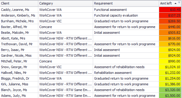
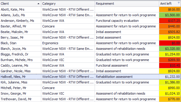
The screen shot below shows what we want to see. To make it obvious, the list has been sorted:
Set up
- If necessary use the Case List Criteria to add a column to the Case List showing the amount left in the estimate. Save the view.
- Right-clicking the Amt left column at the Case List, select Conditional Formatting and then Manage Rules.
The rules manager opens.
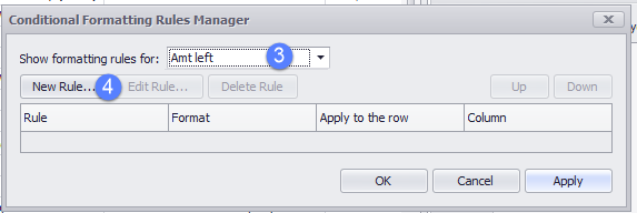
- Select Amt left from the dropdown list.
- Click New Rule.
Add a rule for values under $3000
- Select Format all cells based on their values.
- The three pre-defined condition options for numeric data are now available. Select 3-Color Scale to create a colour scale.
- For the minimum value set the Type to number.
- For the minimum value set the Value to 0.
- For the minimum value click the Colour bar and select a standard red.
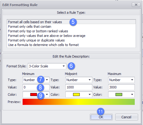
- Repeat step 7 for the midpoint and maximum vales.
- Click OK.
Repeat steps 8-9 for the midpoint and maximum vales, selecting the appropriate colours and values.
You have now made a rule. This new rule doesn't format any values over 3000, so we need a new rule to do that.
Add rule for values over $3000
- Click New Rule again.
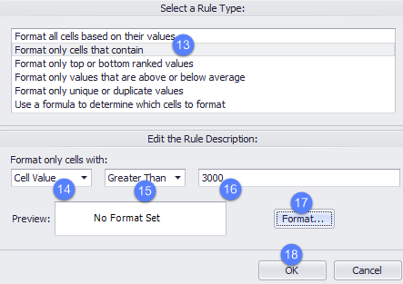
- Select Format only cells that contain.
- Select Cell Value.
- Select Greater Than from the dropdown list.
- Enter 3000.
- Click Format, choose the same standard green as the maximum value at step 10 and click OK.
- Click OK.
You should see your format previewed on the left.
You have now made two rules. You can click Apply to apply them to the Case List or OK to apply them and exit the manager.
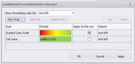
Note that Apply to the row is disabled for the first rule because it is not available with this kind of rule.
You can go back and edit a rule by selecting it and clicking Edit Rule.
The last step is to save your Case List view. The conditional formatting is saved as part of the view.
Result
The screenshot below shows the conditional formatting in action:
Variations
You could vary these rules in several possible ways:
Evaluation of the amount left
- change the values of the three number thresholds to better reflect your requirements
- select Percent rather than Number at step 7 so that cell values are evaluated as a percentage of the maximum value in the whole column (rather than as absolute numbers).
Colours
- make the cell background white rather than green when there is no need to notice it
- achieve a more subtle effect using custom or less saturated colours for the yellow and green and leaving the red fully saturated to indicate danger.
- Change the value of the midpoint colour to change the visual point at which colours start to get 'hotter'.
This involves clicking More colours in the colour screen and selecting the HSB (hue, saturation and brightness) colour model.
Combining conditional formatting with custom columns
This example would be even more useful if the formatting was applied to a custom column displaying Percentage of estimate left.