Conditional formatting
Overview
Conditional formatting helps to visualise information, identify trends and exceptions, highlight critical information and compare data. It is available at the Case List
You set it up by creating one or more rules. Each rule evaluates the contents of particular cells. These cells are usually (but not always) in one column.
Cells are evaluated according to the condition(s) defined in the rule. Cells whose contents meet the criteria are visually formatted to display the result of the evaluation.
This formatting can be applied to the cell or to its entire row.
You can combine multiple formatting rules, including rules comparing the values of cells in different columns.
When the current Saved view is one that you created, your conditional formatting is saved when you save the view. Other local grid operations such as filters are also saved, see Grid filters and saved views.
You can save the current formatting quickly to the current view by clicking the disk icon ![]() at the top of the Case List.
at the top of the Case List.
When the Case List is exported to an Excel file its formatting is also exported, except for the the icon and data bar numeric options, see below.
There are 3 pre-defined conditions that make it easy for you to use conditional formatting:
- Highlight cell rules where ...
- Top/bottom
- Unique/duplicate
The first has an extra option for the evaluation of dates.
There are another 3 pre-defined options that are available only to cells containing numbers.
You can also create conditions from scratch. You can specify more complex evaluations by creating formulae using the Rules Manager.
If desired you can also edit conditional formatting created using the pre-defined conditions. For example, in the rules manager you can customise the formatting.
Simple conditional formatting
To apply simple conditional formatting:
- Right-click the column heading in the Case List and select Conditional formatting from the dropdown list.
- Select one of the three pre-defined conditions.
- Select its option.
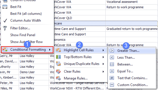
The following pre-defined conditions are available for all columns:
| Highlight Cell Rules | Format where the cell content... |
With this option you will create the condition from scratch by defining how the cell is evaluated. This is more powerful and customisable and involves creating one or more formulae, see Create formula Cells containing dates have an extra option:
See the Dates below |
| Top/bottom rules | Format where the cell value is amongst the... |
This is most useful for numeric data or dates. Cells containing numbers have extra options:
i.e cell value is at least 90% of the maximum column value i.e cell value is 10% or less of the maximum column value |
| Unique/duplicate |
Format where the cell value is:
|
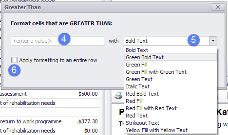
Once you have selected from the options in the table in previous section:
- Enter any value(s) that are appropriate for the condition you selected.
- Select the formatting to be applied from the options in the dropdown list.
- Select whether to apply formatting to the cell or to the entire row that the cell belongs to.
- Click OK.
When you have selected Highlight Cell Rules> A Date Occuring multiple date options are available:
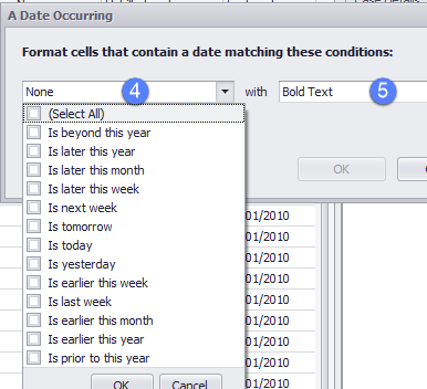
Note that you can click more than one checkbox.
Because these options do not 'compete' with each other, you often have to click more than one. For example, to select all the days this year that are before today, click the following options:
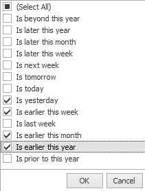
Above you are evaluating whether the date is yesterday or earlier this week or earlier this month or earlier this year. In other words you are evaluating whether the date is any day before today and in the current year.
See Date and time operators for the definitions of these options.
The following additional options are available for cells that contain numbers:
| 4 | Data Bar |
Add a data bar to the cell based on the cell's value |
The longer the bar, the higher is the value at this cell. Various colour options are available. |
||||||||||
| 5 | Colour Scales | Give the cell a background colour based on its value |
The cell's background colour indicates where the cell value falls within a defined range of values: two or three colours Cells colours are continuous graduated between the specified values so they indicate data distribution. Various colour options are available. |
||||||||||
| 6 | Icon Sets | Add an icon to the cell based on its value |
The icon indicates where the cell value falls within a defined range of values. There are several types of icons:
|
Examples of extra options for numerical data
Below is an example of each of the numbered options above:
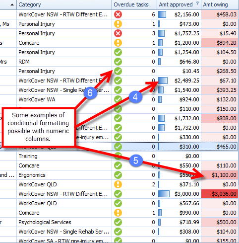
Note:
- With conditional formatting a cell's numeric value can be evaluated as a number or as a percentage of the highest value in the entire column.
As a simple example, we want to format the entire row with a green background for all cases that have any kind of WorkCover Category.
This involves selecting Conditional Formatting from the Category column, then selecting Highlight Cell Rules and Text that Contains:

The text is WorkCover; the Green Fill formatting is selected; and the entire row is checked:

The resulting Case List looks like this:
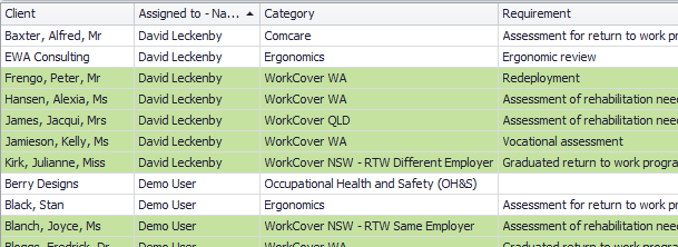
Every case that has WorkCover in its category is displayed with a green background for the entire row.
