
Advanced conditional formatting
It is easy to apply conditional formatting to the Case List by selecting from the standard dropdown options. However, more complex and customisable options are available.
The Conditional Formatting Rules Manager allows you to customise the formatting options, choose from a wider range of standard options and create your own rules.
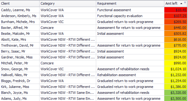
In the example below rules evaluate the contents of the Amt left column.
Cell backgrounds:
- get more red as the amount left gets closer to $0
- are yellow when the amount left is around $1000
- are green when the amount left is >= $3000
 Click image to enlarge/reduce.
Instructions for reproducing this example are at Conditional formatting example.
With the rules manager you can create more complex conditions, including comparing the values in different columns within the same rule.
You create your own evaluation formulae in a similar manner to the Advanced filters with the Filter Editor functionality. You start this either by selecting Highlight Cell Rules > Custom Condition from the pre-defined conditions or by selecting Use a formula to determine cells to format in the rules manager.
Conditional Formatting Rules Manager
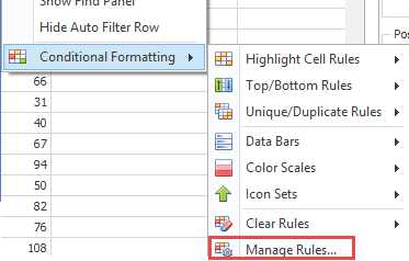
To access the rules manager right-click any column header in the Case List and select Conditional Formatting then Manage Rules....
The rules manager opens and lists any existing conditional formatting rules that you have already created. You can edit them in the manager and customise the formatting to match your specific requirements, including specifying your own colours, typefaces and styles. You can also create new rules that are more complex than the standard options.
A great way to start learning to use the rules manager is to make a formatting rule using one of the pre-defined options and then edit it in the rules manager.
Example
As a simple example, we have a rule where we had selected the Unbilled costs column, created a rule via Highlight Cell Rules > Greater Than and entered the following:
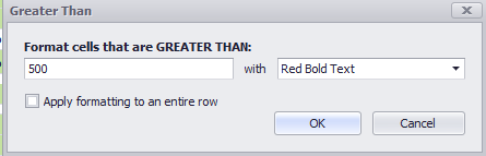
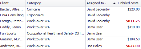
Clearly this rule displays the value of each case's unbilled costs in bold red text if it is over $500:
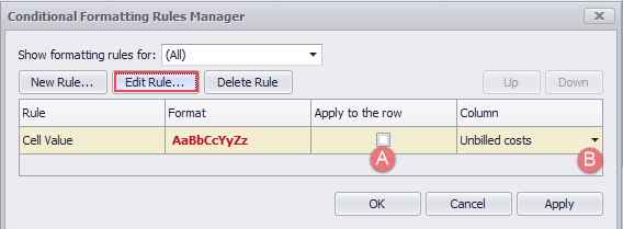
If we open the rules manager via Manage Rules, we will confirm that we have created one rule and it applies to the Unbilled costs column.
- We can change whether its formatting is applied to the entire row.
- We can click the triangle to select from a dropdown list and apply the same evaluation to another column in the current Case List.
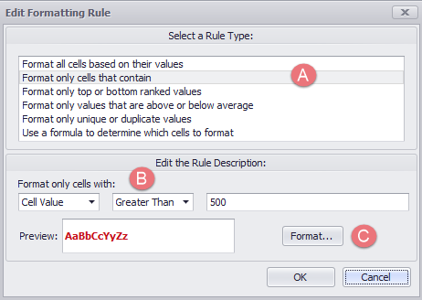
If we click Edit Rule, we see:
- The rule type
- The condition
- A preview of the formatting (bold red text) and an option to click Format... to customise this.
This can be edited.
Note that the last rule type allows you to create a sophisticated boolean formula using the same tools as are available at the Filter Editor.
This can be edited
A broad range of formatting options (colours, typefaces, styles) are available using standard word processing functions.
Create new rule
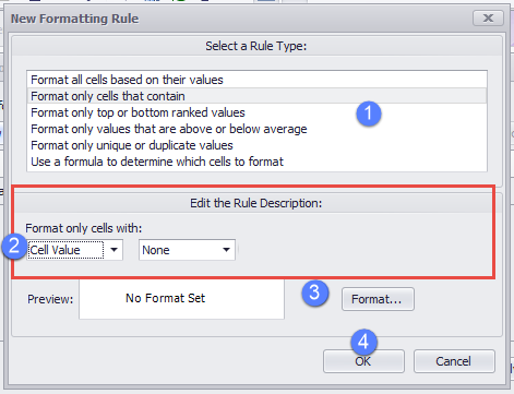
Open the rules manager as above and click New Rule.
- Select the Rule Type
- Select the appropriate evaluation options for the rest of the condition.
- Click Format then specify and save the formatting.
- Click OK
Selecting different options here changes what is seen at sections 2 and 3, see the table below.
A preview is displayed on the left side.
This adds a new rule to the column, by default to the column where the rule manager was launched. You can change this, as explained above.
The Rule Type options at 1 are explained in this table:
| Format all cells based on their values |
This is the equivalent of the three pre-defined conditions for cells containing numbers. Once this is chosen, sections 2 and 3 are replaced by options to customise the formatting and specify any limits required. Note that a cell's numeric value can be evaluated based on its absolute value or its relative value, expressed as a percentage of the highest value in the entire column. |
| Format only cells that contain |
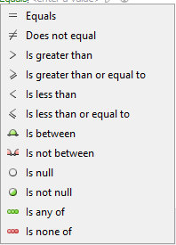
As seen above at 2, you can choose whether the rule evaluates the cell value or the date in the cell. The comparison operations are:
Selecting the date offers a broad range of date comparison options, see Date options at the bottom of this page. |
| Format only top or bottom ranked values | At 2 you nominate how many of the top values you want to format and whether this is an absolute number or a percentage of the maximum value in the column. |
| Format only values that are above or below average |
At 2 you can choose between:
|
| Format only unique or duplicate values |
At 2 you can choose between:
|
| Use a formula to determine cells to format | Select this to open the rule description window and create your own formula, see Create formula below. |
Create formula
Whether you are creating a custom condition or a formula to determine cells to format, you use the same interface and it is very similar to the Advanced filters with the Filter Editor. As with the Filter Editor, you will find this easiest to use if you are technically-minded and are familiar with Boolean operations.
In this window you can create one or more conditions within one rule. They are combined with boolean operations and can also be nested into subgroups.
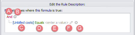
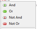
- Click here to select various options. The first four are relevant if you have multiple conditions and want to change their Boolean comparison.
- Click the plus sign to add another condition.
- Click here to select the Case List column to evaluate.
- Click to select the evaluation:
- Enter a value if required
- Click the pencil to change the options at E to other Case List columns. This allows you to compare different column values within the same condition.
- Click the cross to delete a condition.
For example you could create two conditions and state that if either (Or) was true then the cell would be highlighted.
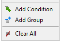
At A you can also select options to add new conditions, add groups to collect conditions together and delete all the conditions:
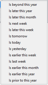
If the column being evaluated contains a date there are additional evaluation options available:
After you have entered the condition(s) click OK and then complete the rule in the usual way by setting the format, specifying whether the whole row is formatted or not and then saving the rule.
Extra options for dates
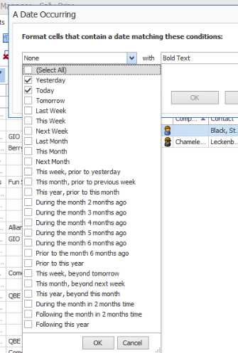
Pre-defined filters for dates are available to the Format only cells that contain Rule Type.
The options are: Yesterday, Today, Tomorrow, Tomorrow, Last Week, This Week, Next Week, Last Month, This Month, Next Month, This week, prior to yesterday, This month, prior to previous week, This year, prior to this month, During the month 2 months ago, During the month 3 months ago, During the month 4 months ago, During the month 5 months ago, During the month 6 months ago, Prior to the month 6 months ago, Prior to this year, This week, beyond tomorrow, This month, beyond next week, This year, beyond this month, During the month in 2 months time, Following the month in 2 months time, Following this year.
You can select multiple options. For example you can target yesterday or today's date:
You may need to include multiple operators because some date and time operators are mutually exclusive, as explained at Date and time operators.
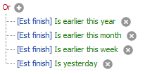
As an example, you are creating a rule in the Rule Editor that looks at the finish date of each case's current estimate. You want to select and highlight any date this year that is before today.
The rule description should contain the following conditions which are compared using the Or operator:
Conditional formatting and custom columns
Conditional formatting comparison operators do not include mathematical operations such as "a particular date plus 5 business days". However custom columns can perform such calculations. See Conditional formatting and custom columns for details.